Open House 2026, Indian Institute of Technology Delhi · October 31, 2026

Microscopy without Lenses Digital Lensless In-line Holographic Microscopy (DLIHM)

Ritish Kamboj and Chhavi Laser Applications and Bio-Imaging Laboratory, Centre SeNSE, IIT Delhi · Supervisor: Prof. Satish Kumar Dubey

Conventional cameras and microscopes form an image by using lenses to project the scene onto a sensor. Lenses make these systems bulky and costly, and the intensity images they record do not reveal the sample's optical thickness (phase).

Computational imaging splits the work differently: the optics only encode the sample into a measurement, and a computer decodes it using a physical model of how light travels. In digital lensless in-line holography we record a diffraction pattern that encodes both the absorption and the phase of the sample, and solving the inverse problem recovers both. The result is a compact, low-cost technique for large field-of-view quantitative phase imaging.

1. Conventional vs computational
2. Diffraction explorer
3. Limits of lens microscopes
4. Working principle
5. Our setup
6. Numerical refocusing
7. Results
8. Pixel super-resolution
9. Applications & FAQ
10. Our lab

Conventional imaging vs computational imaging

In a conventional system the lens does the image formation. In a computational system the hardware only records a measurement, and the image is reconstructed by solving an inverse problem.

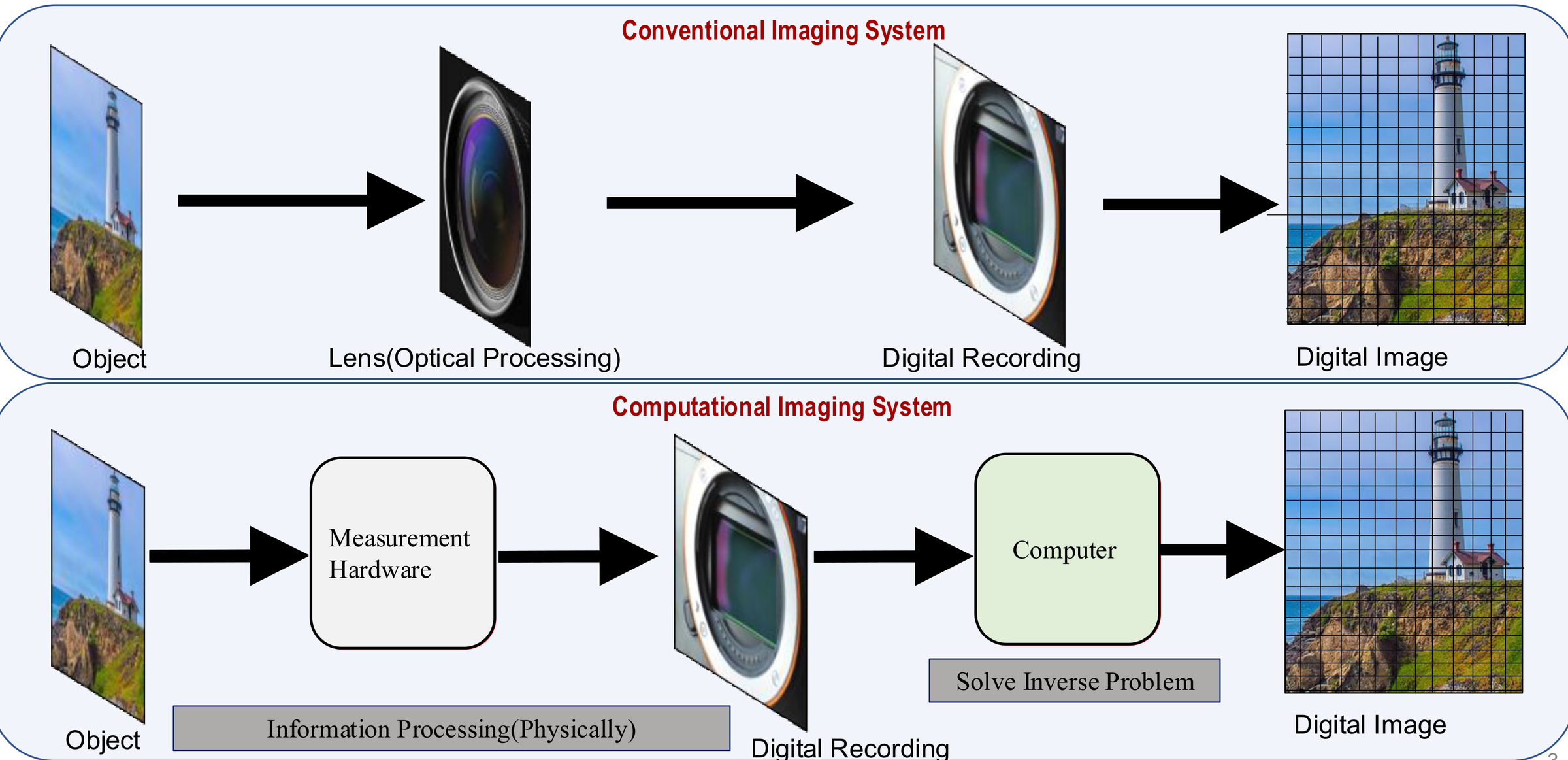
Conventional imaging: object, lens, digital recording, image. Computational imaging: object, measurement hardware, digital recording, computer solving an inverse problem, image. — **Figure 1.** Conventional imaging processes information optically with a lens; computational imaging records a physical encoding of the object and recovers the image numerically.

Conventional vs lensless microscopy

	Field of view	Optics	Phase (thickness)	Size & cost
Conventional microscope	~0.1–2 mm², limited by the objective lens	Objective lenses, precise alignment needed	Not measured (intensity image only)	Bulky, expensive bench-top instrument
Lensless (DLIHM)	~20–30 mm², the entire sensor area	No lenses: LED/laser and a camera chip	Measured quantitatively (optical thickness map)	Compact, low-cost, portable

What the camera actually records

Choose a sample and move the sensor away from it. Close to the sample you see near-field (Fresnel) diffraction, the regime lensless microscopes work in. Far away the pattern turns into far-field (Fraunhofer) diffraction.

Sample-to-sensor distance z = 0 mm

Sample (z = 0)

Camera image at distance z

$Simulated diffraction pattern$

Fresnel number N_F = a²/λz-

Sensor area shown-

Wavelength / pixel535 nm / 1.85 µm

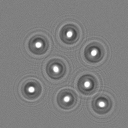
How these images were made: each sample is a complex transmission $A\,e^{i\phi}$ (phase objects are modelled with realistic refractive indices and thicknesses). It is propagated with the band-limited angular spectrum method up to 10 mm and with the Fresnel diffraction integral beyond that. The intensity is integrated over 1.85 µm camera pixels, photon and read noise are added, and every frame is saved as an image. The wavelength and pixel size match our setup. The shaded band on the slider marks the distances used in our experiments and simulations.

Limitations of lens-based microscopes

Why it is worth removing the lens.

Field of view shrinks with magnification

The field of view of an objective falls as its magnification rises. At the magnifications needed to see blood cells it is roughly 0.1–2 mm², so a whole smear has to be scanned field by field with a motorised stage. A lensless sensor sees its full active area (about 20–30 mm²) at once.

Transparent samples are almost invisible

Unstained cells such as red blood cells or microfilariae mostly delay light (a phase shift) rather than absorb it. A bright-field microscope records only intensity, so these samples show little contrast unless they are stained or extra phase-contrast optics are added. A hologram encodes the phase, and the reconstruction measures it quantitatively.

Shallow depth of field

High-numerical-aperture objectives have a depth of field on the order of a micrometre. Cells at slightly different heights are blurred, and refocusing means moving the stage. A hologram records the whole wavefield, so focus can be changed numerically after recording (Section 6).

Size, alignment and cost

Corrected multi-element objectives and precise mechanics make microscopes bulky, alignment-sensitive and expensive, which limits their use outside the laboratory. DLIHM needs only a light source and a camera chip.

Working principle: recording and reconstruction

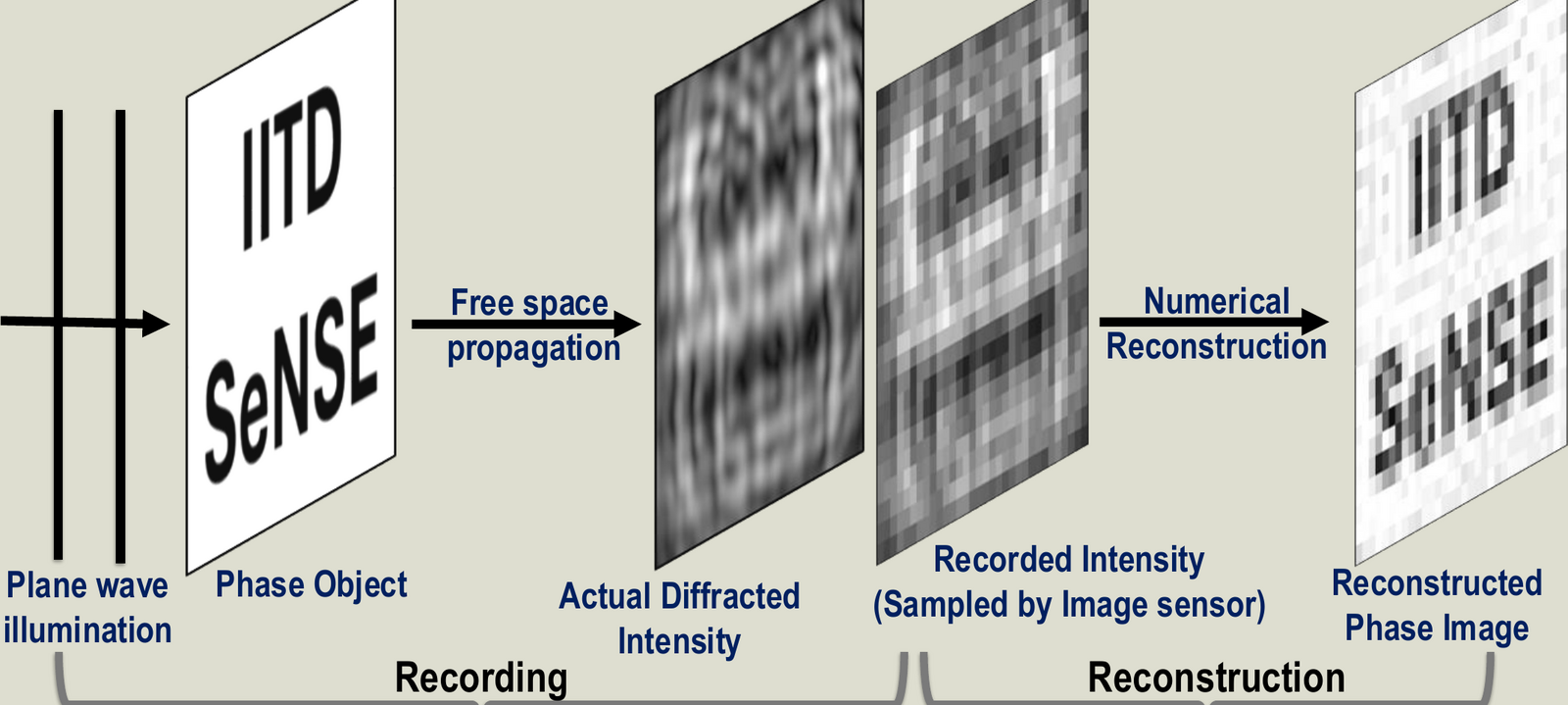
The camera records the intensity of the diffracted light. The image is recovered by solving an inverse problem with a physical model of propagation.

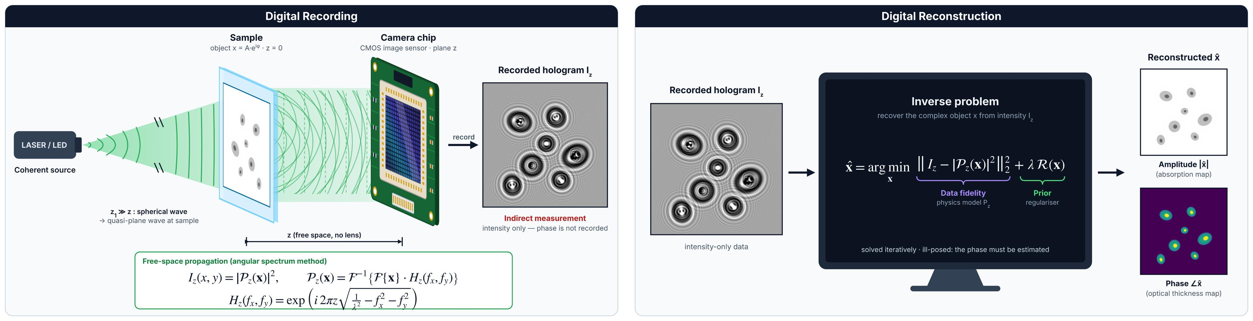
Working principle from the poster: digital recording of a hologram and digital reconstruction by solving an inverse problem to obtain amplitude and phase. — **Figure 2.** Working principle (from our Open House poster). Left: a coherent source illuminates the sample and the camera chip records the hologram $I_z$, an intensity-only, indirect measurement. Right: the complex object is recovered by solving an inverse problem, giving an amplitude (absorption) map and a phase (optical thickness) map.

Forward model

A coherent plane wave illuminates the object $x = A\,e^{i\phi}$ at $z = 0$. Free-space propagation to the camera at distance $z$ is modelled with the angular spectrum method:

$$I_z(x,y) = |\mathcal{P}_z(x)|^2, \qquad \mathcal{P}_z(x) = \mathcal{F}^{-1}\{\mathcal{F}\{x\}\cdot H_z(f_x,f_y)\}, \qquad H_z(f_x,f_y) = \exp\!\left(i 2\pi z\sqrt{\tfrac{1}{\lambda^2} - f_x^2 - f_y^2}\right)$$

Inverse problem

The phase is not recorded, so it has to be estimated. We solve, iteratively,

$$\hat{x} = \arg\min_x \; \big\| I_z - |\mathcal{P}_z(x)|^2 \big\|_2^2 + \alpha\,\mathcal{R}(x)$$

The first term keeps the estimate consistent with the measurement (data fidelity through the physics model). The regulariser $\mathcal{R}$ adds prior knowledge about the sample. The amplitude $|\hat{x}|$ gives the absorption map and the phase $\angle\hat{x}$ gives the optical thickness map.

Two difficulties

Lost phase and the twin image. The sensor records only intensity. Simply back-propagating the hologram overlays the in-focus image with an out-of-focus "twin image", which corrupts both amplitude and phase. Phase retrieval with constraints and regularisation suppresses it.

Pixel size limits resolution. With the sample close to the sensor, the finest diffraction fringes are smaller than the 1.85 µm pixels. They are averaged and aliased during recording, so resolution is set by the pixel pitch. Section 8 shows how we address this.

Our setup

A light source, the sample, and a bare camera sensor a few millimetres below it. There are no lenses between sample and sensor.

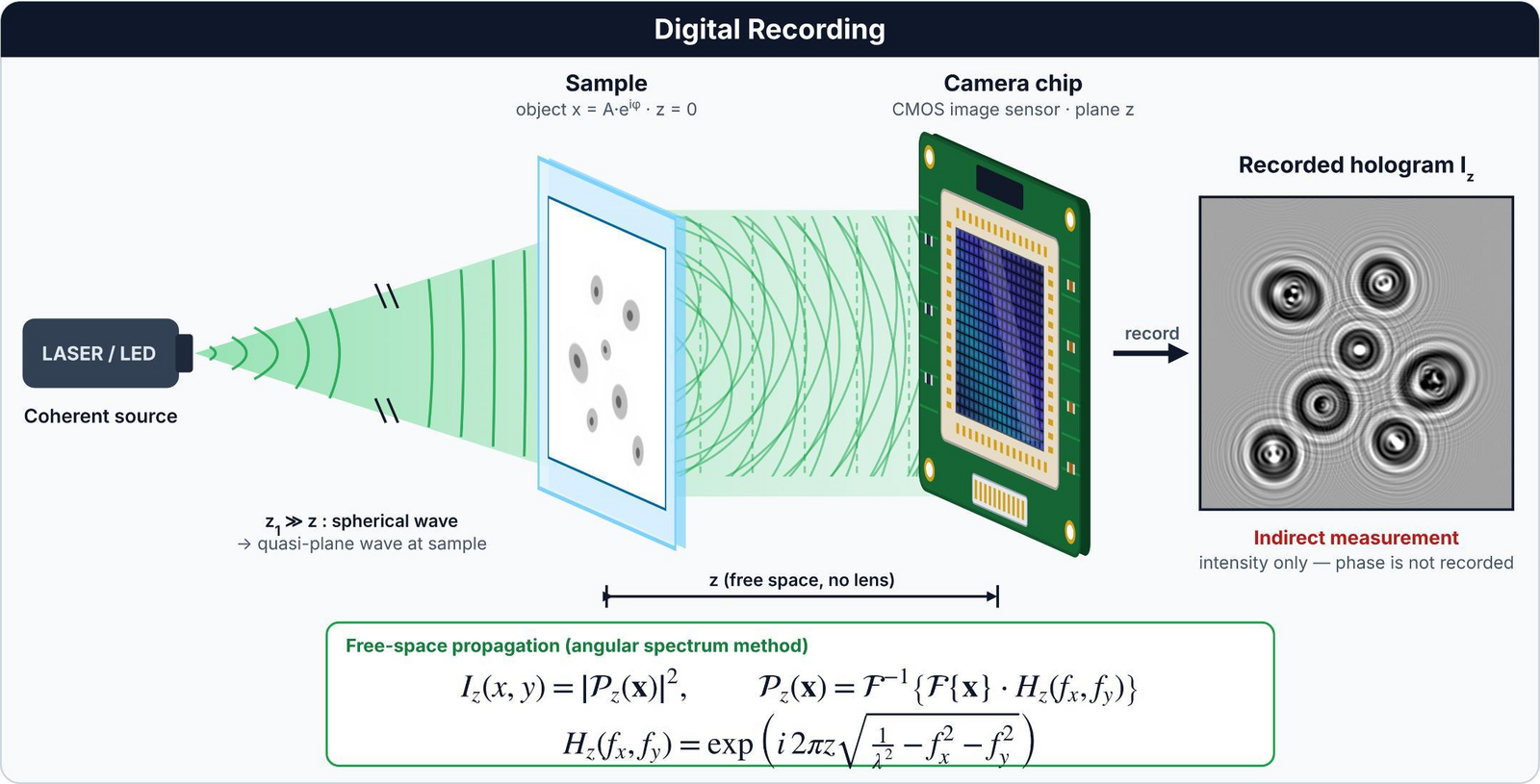
Recording geometry: laser or LED source, sample at z = 0, camera chip at distance z, recorded hologram. — **Figure 3.** Recording geometry. The source is far from the sample compared with the sample-to-sensor distance $z$, so the sample is illuminated by a quasi-plane wave.

Illumination	Coherent source (laser / LED), wavelength 535 nm
Camera	CMOS sensor, 4000 × 3000 pixels (12 MP), pixel pitch 1.85 µm
Sample-to-sensor distance	A few millimetres; our USAF-chart recordings used 4.45–6.02 mm
Imaging optics	None between sample and sensor
Recording	A single hologram, or several holograms at different sample-to-sensor distances for multi-height phase retrieval (for example 12 holograms between 6 and 7.2 mm, 0.1 mm apart, for the USAF chart)

Numerical refocusing and autofocus

A hologram can be back-propagated to any plane, so focusing becomes a computation instead of a knob. To find the sample plane automatically we look for the plane where the total variation (TV) of the reconstruction is lowest.

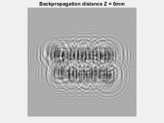Back-propagated reconstruction at the selected distance

defocused

Back-propagations of a simulated in-line hologram of a text target placed 10 mm from the sensor, computed for 27 distances between 0 and 20 mm.

Back-propagation distance 0 mm

TV of the back-propagated field, computed between 6 and 14 mm (values ×10⁶). The sharp minimum at 10 mm is the object plane.

Experimental results

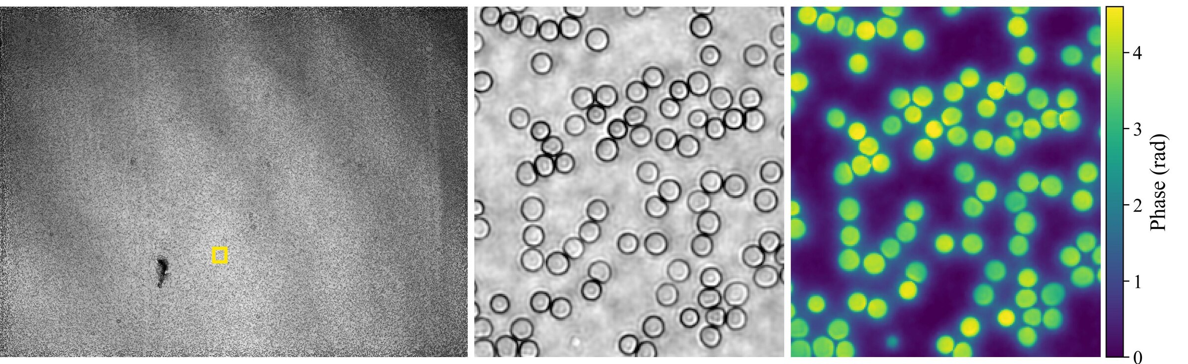
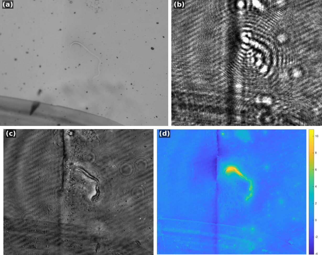
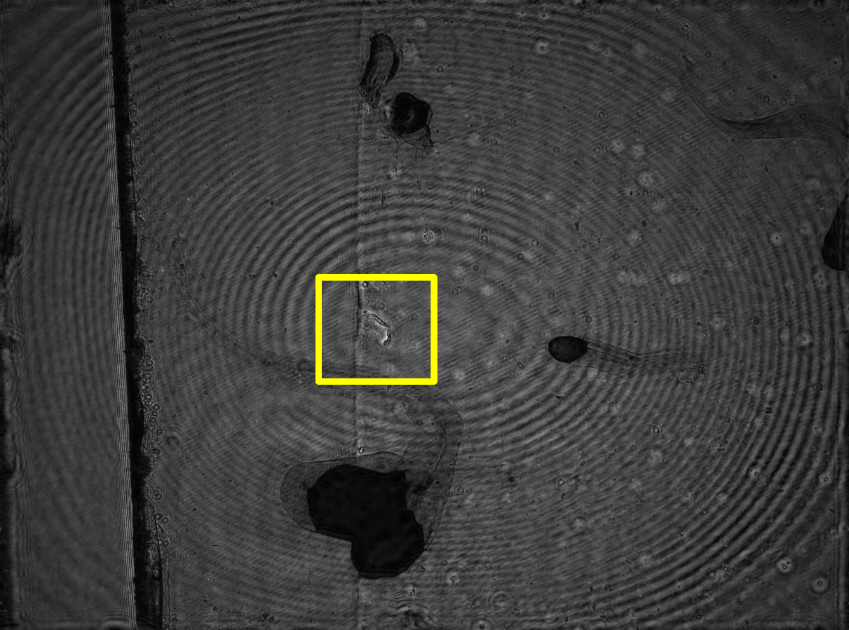
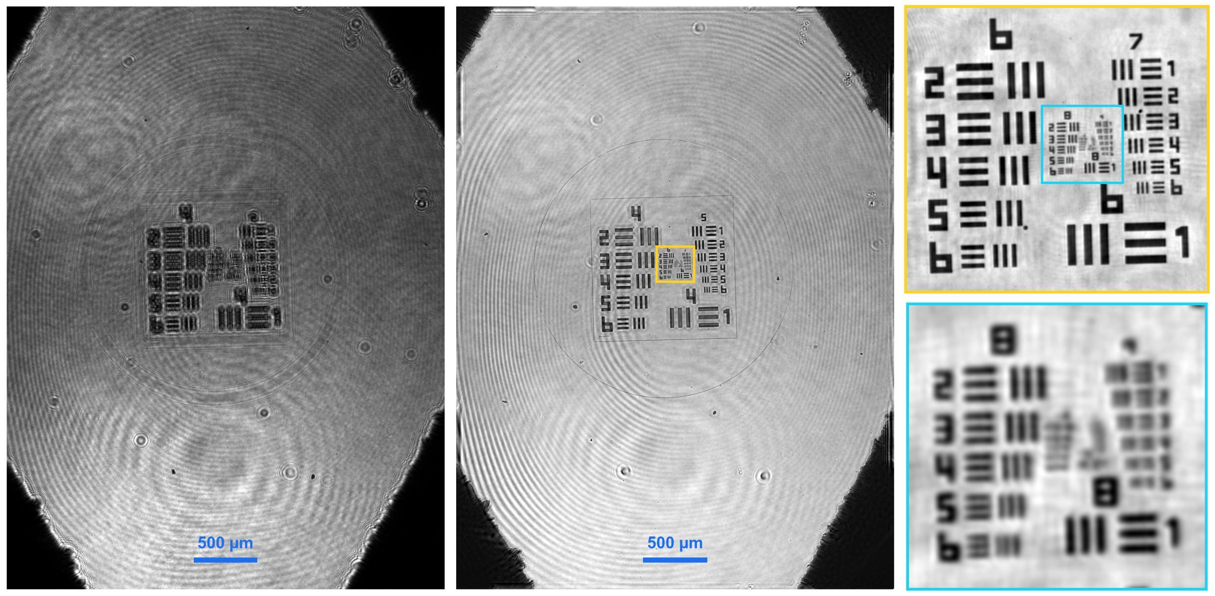
Holograms recorded with our lensless setup and their reconstructions. Click a figure to enlarge it.

Reconstructed absorption map of a blood smear with an enlarged region, and the reconstructed phase map of red blood cells. — **Human red blood cells (blood smear).** Left: reconstructed absorption map of the field of view; the yellow box marks the region shown enlarged in the middle. Right: reconstructed phase map (radians). The cells are imaged without staining, and the phase map gives each cell's optical thickness.

Microfilaria: bright-field image with a 10x objective, recorded lensless hologram, reconstructed amplitude, and phase map. — **Unstained microfilaria.** (a) Conventional bright-field image (10× objective): the transparent parasite has poor contrast. (b) Recorded in-line hologram (lensless). (c) Reconstructed amplitude. (d) Corresponding phase map.

Large field-of-view lensless image of the microfilaria sample with a yellow rectangle marking the field of view of a 10x objective. — **Large field of view.** Lensless image of the same unstained microfilaria sample. The yellow rectangle marks the field of view of a conventional 10× objective, far smaller than the full sensor area.

USAF 1951 chart: recorded hologram and reconstructed image with 500 micrometre scale bars, and two magnified insets. — **USAF 1951 resolution chart.** Left: recorded hologram. Centre: reconstructed image (scale bars 500 µm). Right: magnified views of the regions marked by the yellow and cyan boxes, containing the smallest bar groups.

Beating the pixel limit with a single hologram

Our work on single-shot pixel super-resolution for DLIHM, published in Applied Optics.

Applied Optics 65(18), 6093–6103 (2026)

Single-shot pixel super-resolution lensless in-line holographic microscopy using object support constraints

Ritish Kamboj, Balpreet Singh Ahluwalia, Satish Kumar Dubey

doi.org/10.1364/AO.598994 Read the paper (PDF)

The problem

Placing the sample close to the sensor gives a wide field of view, but the finest diffraction fringes are then smaller than a camera pixel. Each pixel averages them, frequencies above the Nyquist limit $1/(2\Delta p)$ alias, and resolution is limited by the pixel pitch rather than by diffraction. Existing pixel super-resolution methods record several holograms (shifted source, sample or sensor; several heights; several wavelengths). That needs extra hardware and precise registration, and it sacrifices temporal resolution.

Question: can a finite object support, combined with recording the diffraction pattern over an area larger than the object, give enough information to recover sub-pixel detail from a single, heavily undersampled measurement?

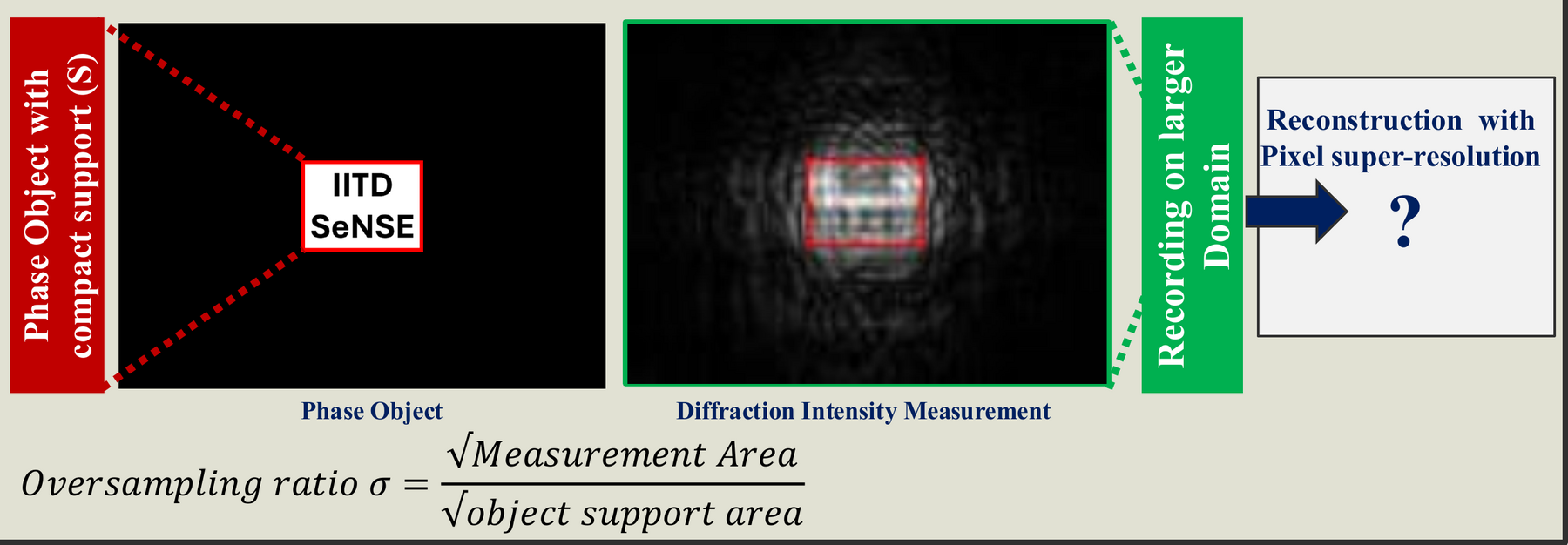
Phase object with compact support, its diffraction intensity measurement recorded on a larger domain, and the question of reconstruction with pixel super-resolution. Oversampling ratio defined as square root of measurement area over object support area. — **Problem statement.** A phase object with compact support $S$ is recorded over a larger domain. The oversampling ratio $\sigma = \sqrt{\text{measurement area}}/\sqrt{\text{object support area}}$ measures how much larger.

Theory: a pixel-aware forward model

Plane wave illuminates a phase object; free-space propagation gives the actual diffracted intensity; the image sensor records a pixel-sampled intensity; numerical reconstruction gives the phase image. — The sensor does not record the true diffraction intensity, only its pixel-averaged version. The reconstruction has to account for that.

Each pixel integrates the intensity over its area, which we model with a binning operator $\mathcal{B}_b$ that averages $b\times b$ blocks of a fine computational grid. With the object restricted to its support $S$, the measurement is

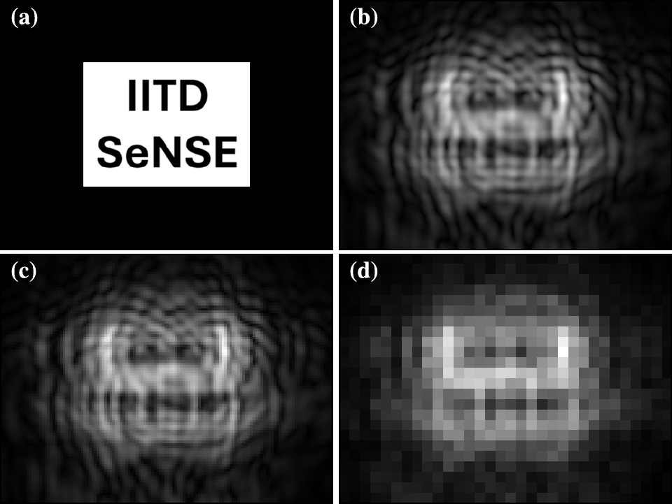
$$I_z^{(b)} = \mathcal{B}_b\big(|\mathcal{P}_z(O \odot S)|^2\big)$$

Finite-support phase object, its high-resolution hologram, and the same hologram binned by factors 4 and 16. — (a) Phase object with finite support, (b) its high-resolution hologram, (c, d) the same hologram binned by $b = 4$ and $16$: fine fringes are lost.

Why this can work: an object with compact support has a Fourier transform that is an entire analytic function, which is determined by its values over any finite region. Free-space propagation spreads the object's high spatial frequencies across the measurement plane, so they are encoded in the fringes, including fringes beyond the object's own extent.

Recording over a larger area raises the measurement-to-unknown ratio

$$\eta = \frac{N_\text{meas}}{N_\text{unknown}}$$

which stabilises the inversion.

The object is recovered on a fine grid by minimising

$$O^* = \arg\min_{O}\; \frac{1}{2}\Big\| \sqrt{I_z^{(b)}} - \sqrt{\mathcal{B}_b\big(|\mathcal{P}_z(O\odot S)|^2\big)} \Big\|_2^2 + \alpha\,\mathrm{TV}(O)$$

using a monotone FISTA (accelerated gradient) scheme with projection onto the support after every step. We call the method SCAR-PSR (support-constrained aliasing-reduction pixel super-resolution). The baseline, NU-PSR, uses the same optimiser and support constraint but up-samples the measurement and ignores pixel integration.

Results (numerical study)

Simulation parameters: wavelength 500 nm, 0.25 µm computational grid, phase range 0–π/2, propagation distances 0.35–0.6 mm.

Simulated object, NU-PSR and SCAR-PSR reconstructions for oversampling ratios of 4 and 8. — **Effect of recording area.** 16× binning (4 µm effective pixels), $z = 0.5$ mm. Top row $\sigma = 4$, bottom row $\sigma = 8$. (a, d) Support-limited object, (b, e) NU-PSR, (c, f) SCAR-PSR. With the larger recording window SCAR-PSR recovers the fine features even from this heavily undersampled data.

USAF chart phase: high-resolution ground truth, SCAR-PSR reconstruction, low-resolution ground truth at camera resolution, and line profiles of group 10. — **Resolution with a USAF phase chart.** 8× binning (2 µm effective pixels), $z = 0.6$ mm. (a) High-resolution ground truth, (b) SCAR-PSR reconstruction, (c) ground truth at camera resolution, where features finer than group 8 element 1 are not resolved. (d) Line profiles through group 10. SCAR-PSR resolves up to group 10 element 3, a line width of about 0.4 µm: roughly a 5× gain over the native sampling.

Cameraman and gravel phase images: ground truth, binned low-resolution image, and SCAR-PSR reconstruction. — **Natural (non-binary) phase objects.** 4× binning (1 µm effective pixels), $z = 0.6$ mm, $\sigma = 8$. (a, d) Ground-truth phase, (b, e) the object at camera resolution, (c, f) SCAR-PSR reconstruction recovering features finer than the camera resolution.

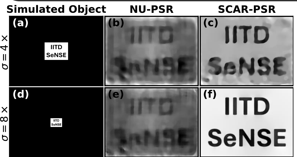
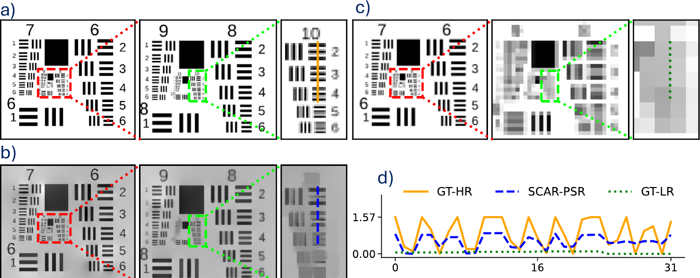
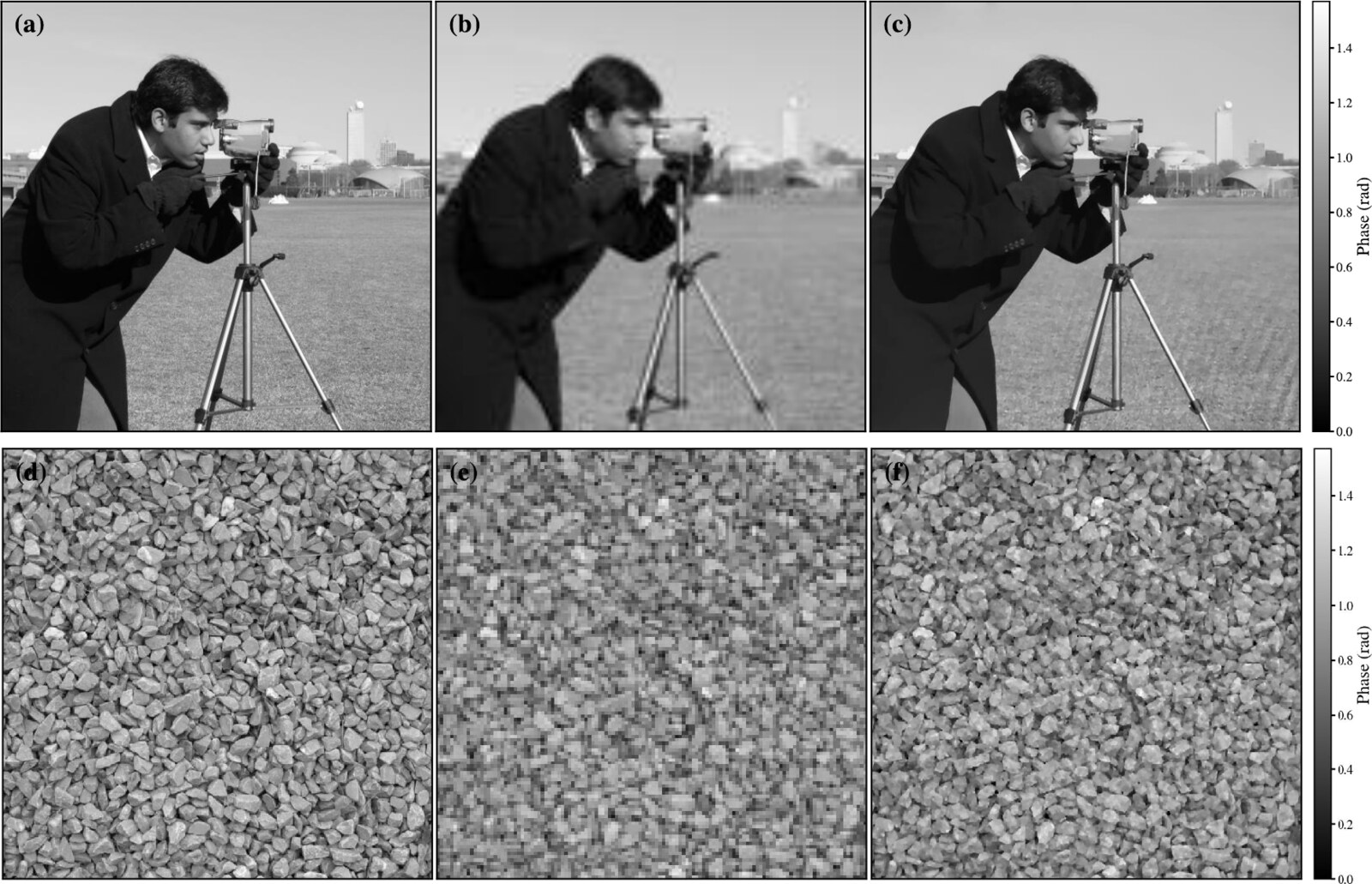
Key numbers

8× binning (2 µm pixels)	Phase SNR	PCC	SSIM
NU-PSR (no pixel model)	12.57 dB	0.9719	0.5285
SCAR-PSR	24.1 dB	0.9981	0.9128

Half-period resolution of 0.4 µm from 2 µm effective pixels (coherent diffraction limit λ/2 = 0.25 µm).
Stable reconstruction down to about 500 photons per pixel; phase SNR saturates near 24 dB from six-bit detector precision upward.
Support constraints alone are not enough. The pixel-integration model is what makes single-shot super-resolution stable.

These results are numerical. Experimental validation and dynamic biological imaging are the next steps. The method needs the sample to be compact compared with the sensor area, i.e. it trades field of view for resolution.

Applications and frequently asked questions

Point-of-care diagnostics

Blood cell counting and microfilariae screening from a single wide-field recording, without stains.

Label-free cell monitoring

Live-cell and cell-culture monitoring through quantitative phase, without fluorescent labels.

Water quality

Detection of microplastics and plankton in water samples.

Education and field use

A low-cost, lens-free microscope for teaching laboratories and field settings.

FAQ

Why does light diffract around a cell?

By the Huygens–Fresnel principle every point of a wavefront acts as a source of secondary wavelets. When light meets a structure only a few wavelengths across (a 7–8 µm red cell versus 0.535 µm light), these wavelets interfere and form rings and fringes instead of a sharp shadow. Section 2 shows how the pattern evolves with distance.

What is the twin-image problem?

The sensor records $I = |R + O|^2$, the intensity of the unscattered reference $R$ plus the light scattered by the object $O$. Back-propagating this intensity brings the object into focus but also produces its complex conjugate, an out-of-focus "twin" on the same axis. Iterative phase retrieval with constraints (for example, object support) and regularisation suppresses it.

How can focus be changed without moving anything?

The hologram contains the whole wavefield, so the field at any plane can be computed by multiplying its spectrum by the free-space transfer function $H_z(f_x,f_y) = \exp\!\big(i2\pi z\sqrt{\lambda^{-2} - f_x^2 - f_y^2}\big)$. Sweeping $z$ and picking the plane with minimum total variation finds the sample automatically (Section 6).

How does single-shot super-resolution recover detail finer than a pixel?

If the object occupies a known, limited region and the hologram is recorded over a larger area, there are more independent measurements than unknowns. Modelling exactly how each pixel averages the intensity lets the reconstruction undo that averaging and recover aliased high-frequency information. In simulation this gives about a 5× resolution gain (Section 8).

Documents

Open House poster (PDF) Applied Optics paper (PDF)

Our lab

The Laser Applications and Bio-Imaging Laboratory at Centre SeNSE, IIT Delhi works where laser technology meets biological imaging, with the aim of advancing medical diagnostics and scientific research.

Principal investigator

Prof. Satish Kumar Dubey

Professor, Centre for Sensors, Instrumentation and Cyber-Physical System Engineering (SeNSE), Indian Institute of Technology Delhi, New Delhi 110016

Email: satishdubey@sense.iitd.ac.in
Phone: +91-11-2659 6752

Lab website Google Scholar ORCID LinkedIn

Current projects

Field-portable lensless microscope for filariasis detection, funded by BIRAC. The holographic microscope on this page is developed under this project, with AIIMS Nagpur, CDAC Kolkata and CSTM Kolkata as collaborators. It was showcased at Global Bio India 2024, Bharat Mandapam, New Delhi (12–14 September 2024).
Point-of-care device: a smartphone-based device for early diagnosis of chronic kidney disease.
Surface-enhanced Raman spectroscopy (SERS): detection of urinary and salivary cotinine.

More on the lab's people, publications, patents and projects: web.iitd.ac.in/~satishdubey